Portfolio Management
MGMT 648 · October 10
Sat Oct 10, 2026
The Sharpe ratio
Excess return per unit of standard deviation.
Definition
The numerator is the average excess return: what the investment earned beyond a Treasury bill. The denominator is the standard deviation of that same excess return, which equals the standard deviation of the return itself when the bill rate is known in advance.
Can be regarded as reward per unit risk.
Cash
Cash is invested at the money market rate . Suppose half of each dollar invested is put in stocks earning and the other half is in the money market. The portfolio return and the excess return over the money market rate are
The expected excess return and the standard deviation are each half those of , so the Sharpe ratio is the same as that of . This fact is true for any division between stocks and the money market.
Leverage
If we invest $100 and borrow another $100 at the rate to hold $200 of stocks, then the portfolio return and excess return are:
The expected excess return and the standard deviation are each twice those of , so the Sharpe ratio, measured against the borrowing rate, is again the same. This is true for any amount borrowed.
Simplification
To simplify, we will assume borrowing and saving at the T-bill rate. In reality, brokerages charge more than that for borrowing.
Some ETF data
Returns
Total returns on three sheets: weekly, monthly, and annual.
Sample
January 2005 through October 2026. GLD has the shortest history of these funds; it began trading in November 2004.
Risk-free rate
The 3-month Treasury, FRED series DGS3MO. It averaged 1.8% over the sample and pays 4.2% today.
Download: etf_returns.xlsx. Every optimization that follows uses the monthly sheet; the weekly sheet is what the estimation-error slides discuss.
One portfolio, three leverages
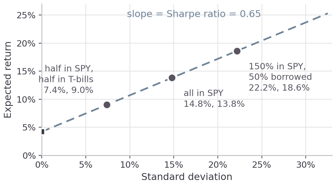
Each point is a combination of SPY and Treasury bills. The line starts at the bill rate and its slope is the Sharpe ratio, so raising the Sharpe ratio tilts the whole line up and gives a higher average return at every level of risk.
We’re assuming borrowing at the T-bill rate. In reality, there will be a 1% or 2% spread. That changes the slope, bending the line down, beyond the “all in” point.
Two funds: IEF and SPY
The two funds
IEF
iShares 7–10 Year Treasury Bond ETF. Holds Treasury notes with seven to ten years left to maturity and sells them as they age out of that range. No credit risk; the price moves when yields move.
SPY
SPDR S&P 500 ETF Trust. Holds the 500 stocks of the S&P 500 in index proportions. Listed in 1993, the first US exchange-traded fund.
Excess returns, not raw returns
Every mean and standard deviation from here on is estimated from excess returns: returns minus the T-bill return for that period.
IEF
Over the sample, IEF averaged 3.1% a year, and T-bills averaged 1.8%, so the premium was 1.3%. It makes more sense to extrapolate the 1.3% premium to the future than to extrapolate the 3.1% mean return, because T-bills today are at 4.2%: the expected return is 5.5%.
Treasuries and the S&P 500
| Average excess return | Standard deviation | Sharpe ratio | Expected return | |
|---|---|---|---|---|
| IEF, 7–10 year Treasuries | 1.3% | 6.5% | 0.20 | 5.5% |
| SPY, S&P 500 | 9.6% | 14.8% | 0.65 | 13.8% |
The correlation between the two is .
Monthly excess returns, 261 months, annualized. Expected return is today’s 4.2% plus the average excess return, and is the vertical axis of every picture that follows.
Maximizing the Sharpe ratio
Choose the weights on the funds to make the Sharpe ratio as large as possible. The weights should sum to 1 (fully invested in the two ETFs with no leverage).
Prompt
Find the portfolio of IEF and SPY that maximizes the Sharpe ratio. Use the monthly returns in etf_returns.xlsx to estimate means, standard deviations, and the correlation. Use a risk-free rate of 0.042/12. Do you need any other information from me?
I expect it to ask whether you want to allow short sales. Say “yes.” When it finishes, ask for a plot, if it didn’t give you one automatically.
Every mix of the two
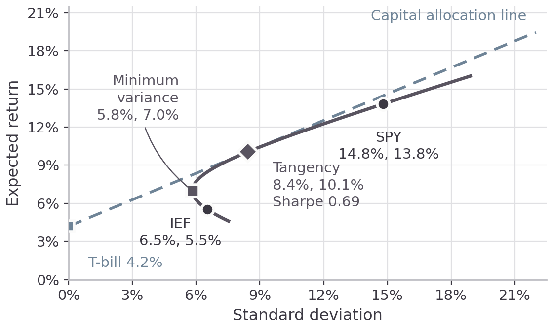
The minimum-variance portfolio
The left tip of the curve: the weights that make the portfolio’s standard deviation as small as possible. Nothing is said about its average return, and that missing condition is what separates it from the problem on the next slide.
82% IEF
18% SPY
5.8% standard deviation
At 5.8% it carries less risk than IEF alone, which is 6.5%, and earns more over bills: 2.8% against 1.3%.
The tangency portfolio
45% IEF
55% SPY
0.69 Sharpe ratio
Neither fund on its own reaches 0.69. SPY alone is 0.65 and IEF alone is 0.20.
A third fund: GLD
Gold against the other two
| Average excess return | Standard deviation | Sharpe ratio | Expected return | |
|---|---|---|---|---|
| IEF | 1.3% | 6.5% | 0.20 | 5.5% |
| SPY | 9.6% | 14.8% | 0.65 | 13.8% |
| GLD | 9.6% | 17.3% | 0.56 | 13.9% |
Correlations: GLD with SPY 0.08, GLD with IEF 0.31, IEF with SPY .
What does GLD add?
GLD and SPY have the same average excess return, 9.6%, and GLD is the more volatile of the two: 17.3% against 14.8%.
What GLD adds
Its correlation with the 45/55 portfolio of IEF and SPY is 0.19. SPY’s correlation with that same portfolio is 0.94.
The criterion
An asset is worth holding when its excess return is high relative to its covariance with the portfolio, not relative to its own variance.
Exercise
Use AI to find the minimum variance portfolio and the tangency portfolio using the monthly returns to estimate means, variances, and covariances. Assume the risk-free rate is 0.042/12. If asked about short sales, tell AI to allow them (it won’t matter for this example).
Ask for a plot.
The new weights
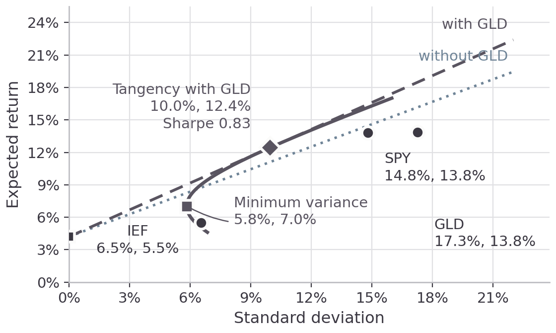
17% IEF
50% SPY
33% GLD
The Sharpe ratio rises in sample from 0.69 to 0.83. The minimum-variance portfolio hardly moves — 5.8% either way, with well under 1% in GLD — so the gain is in the tangency portfolio and not in the left tip.
In sample, because these are the weights that fit this sample best. What they earn on returns they were not fitted to comes at the end of this half.
Three funds
How precisely we know the inputs
Confidence intervals for means and for standard deviations.
Annualizing means and standard deviations
A year’s return is the sum of 52 weekly returns, exactly in logs and closely enough in levels. If those 52 returns are independent of one another, the variance of their sum is the sum of their variances:
Means add the same way, , so the mean scales with the number of periods and the standard deviation with its square root.
The independence assumption
SPY’s weekly excess returns have a lag-1 autocorrelation of , so part of each week’s move is reversed the week after. Some of the weekly variance cancels inside a month, and the variance of a monthly return comes to 3.06 times the variance of a weekly return rather than 4.33.
17.6% annualized from weekly
14.8% annualized from monthly
17.1% from annual returns
The third number breaks the pattern, and two things are behind it. Monthly returns are mildly positively autocorrelated, at lag 1, which pushes the annual variance above 12 times the monthly. But that accounts for only about a seventh of the gap. The rest is that 21 observations cannot pin down a standard deviation at all.
This is why every optimization in this session runs on monthly returns. A weekly covariance matrix scaled by 52 overstates the annual risk of whatever reverses week to week, and the optimizer prices that overstatement into its weights.
Confidence intervals, from annual data
With annual excess returns drawn from a distribution with standard deviation , the sample average has standard error , and the 95% interval for the expected excess return is
At and years the standard error is 3.7%, so the interval runs 7.3 points either side of the average. Halving that width takes four times the years; getting it to a point either side would take about 1,100.
The mean at three frequencies
| Returns | Observations | Average excess | Standard deviation | Standard error | 95% interval |
|---|---|---|---|---|---|
| Annual | 21 | 10.30% | 17.08% | 3.73% | 3.00% to 17.61% |
| Monthly | 252 | 0.789% | 4.274% | 0.269% | 0.262% to 1.317% |
| Weekly | 1,095 | 0.191% | 2.445% | 0.074% | 0.046% to 0.336% |
The annual row is already annual. Multiply the monthly row by 12 and the mean is 9.5% a year, the interval 3.1% to 15.8%; multiply the weekly row by 52 and the mean is 9.9%, the interval 2.4% to 17.5%. There is very little difference. More frequent observations do not help in estimating annual means.
The standard deviation at three frequencies
| Returns | Observations | Standard deviation | 95% interval |
|---|---|---|---|
| Annual | 21 | 17.08% | 13.07% to 24.67% |
| Monthly | 252 | 4.274% | 3.931% to 4.684% |
| Weekly | 1,095 | 2.445% | 2.346% to 2.552% |
Multiply the monthly row by and the standard deviation is 14.8% with a confidence interval of 13.6% to 16.2%. More frequent observations help a great deal in estimating standard deviations.
Annualizing the weekly row (multiply by ) produces an estimate that is too high (17.6%), because it ignores the weekly reversals.
Correlations
There is a correlation to be estimated for each pair of assets. That makes correlations for assets. For the S&P 500, we have
500 means
500 variances
124,750 correlations
Three funds took nine numbers. The S&P 500 takes 125,750, each one carrying a confidence interval.
Treat the output of a mean-variance optimizer with a lot of skepticism, particularly for a large number of assets.
Short sales
Negative weights, margin, and the rebate.
Nothing requires a weight to be positive
A negative is a short sale.
- Borrow the shares from another investor, through your broker.
- Sell them. The proceeds stay in the account as collateral for the loan.
- Buy the shares back later and return them.
You owe the lender any dividends paid while you are short, so what you pay over the life of the position is the total return on the stock.
Regulation T
The Federal Reserve sets initial margin at 50% of market value for a purchase and 50% on top of the proceeds for a short sale.
The constraint
Required equity is half the long position plus half the short position, so long + short can be at most twice your equity.
A 130/30 fund
130 long and 30 short is 160 of gross exposure against 100 of equity, inside the Reg T limit of 200.
FINRA sets the maintenance requirement afterwards: 25% of a long position and usually 30% of a short one.
The short interest rebate
The lender holds your sale proceeds as cash collateral and invests them. The interest paid back to you is the rebate.
General collateral
Easy-to-borrow shares. The loan fee is a few basis points, so the rebate is close to the full market rate.
Specials
Hard-to-borrow shares. The fee can exceed the market rate and the rebate turns negative.
Retail accounts
The broker often keeps the interest on the proceeds and the rebate is zero.
Everything that follows assumes a 100% rebate: the proceeds earn the full risk-free rate.
What a long-short strategy earns
Invest $1. Go long dollars and short dollars. With a full rebate, you earn on .
Set (the fraction invested in ) and set (a negative number representing your investment in ). Then you earn on . The portfolio return and excess return are
This is the same arithmetic as for two long positions, just with being negative.
Another example: Add real estate and international stocks
Two more funds
Add these to IEF, SPY and GLD.
| Ticker | Fund |
|---|---|
| VNQ | Vanguard Real Estate |
| EFA | iShares MSCI EAFE, developed markets outside North America |
Ask for the tangency portfolio with short sales allowed, using the monthly returns to estimate means, variances, and covariances. Then ask for it when short sales are disallowed. Use a risk-free rate of 0.042/12.
Constraining the weights
In sample, constraints hurt performance. But constraints can produce better out of sample behavior. Constraints can reduce “overfitting” to a particular random sample.
There are other methods to reduce overfitting: push the expected return and risk estimates all closer to each other or shrink all weights towards market weights.
For strategic asset allocation &mdash deciding on a baseline allocation to asset classes &mdash people never allow short sales.
One more example: Industry sectors
Nine sector funds
Ask for tangency portfolios without short sales for these funds, using the monthly returns in sector_returns.xlsx to estimate means, variances, and covariances. Use a risk-free rate of 0.042/12. Interpret the weights &mdash why high allocations to some sectors and low allocations to others.
| Ticker | Sector | Ticker | Sector |
|---|---|---|---|
| XLB | Materials | XLP | Consumer staples |
| XLE | Energy | XLU | Utilities |
| XLF | Financials | XLV | Health care |
| XLI | Industrials | XLY | Consumer discretionary |
| XLK | Technology |
MGMT 648 · Applied Finance